Time complexity is one of the most important concepts in Data Structures and Algorithms. It helps you understand how an algorithm behaves as the input size grows and why some solutions fail to scale.
This guide explains time complexity step-by-step using simple explanations and Python examples written purely as text, focusing on intuition rather than heavy mathematics.
1. What Is Time Complexity?
Time complexity measures how the running time of an algorithm grows as the input size increases.
It does not measure actual seconds taken by the program.
Instead, it focuses on how fast execution grows relative to input size n.
The focus is on growth rate, not machine speed.
2. Why Time Complexity Matters
Time complexity helps you:
- Compare different algorithms
- Predict performance for large inputs
- Perform better in coding interviews and competitive programming
- Avoid inefficient solutions early
Efficient code is essential for scalable real-world systems.
3. Asymptotic Notations
Big O (O)
Represents the worst-case time complexity.
It is the most commonly used notation in interviews.
Big Ω (Omega)
Represents the best-case time complexity.
Big Θ (Theta)
Represents the average-case time complexity.
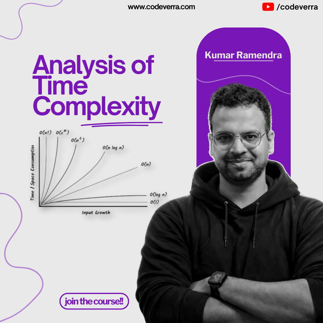
4. Common Time Complexities (Overview)
O(1) – Constant
O(log n) – Logarithmic
O(n) – Linear
O(n log n) – Linearithmic
O(n²) – Quadratic
O(2ⁿ) – Exponential
5. O(1) — Constant Time
Explanation
The execution time does not depend on the input size.
Python Example (Text Only)
A function that returns the first element of an array always runs in constant time, regardless of how large the array is.
For example:
def get_first_element(arr):
    return arr[0]
This is the fastest possible time complexity.
6. O(log n) — Logarithmic Time
Explanation
The input size is reduced by half in every step.
Python Example (Binary Search – Text Only)
Binary search repeatedly divides the search space into two halves.
Example logic:
Initialize low and high pointers.
Find the middle element.
Compare the middle element with the target.
Discard half of the array in each step.
Because the input is halved every time, the complexity is O(log n).
7. O(n) — Linear Time
Explanation
Execution time grows directly proportional to input size.
Python Example (Text Only)
Finding the maximum element in an array requires checking every element once.
Example logic:
Initialize maximum with the first element.
Traverse the array.
Update maximum whenever a larger value is found.
If the input size doubles, execution time also doubles.
8. O(n log n) — Linearithmic Time
Explanation
This complexity appears in efficient sorting algorithms.
Python Example (Merge Sort Idea – Text Only)
Merge sort divides the array into halves recursively and then merges them.
Divide step takes log n time.
Merge step takes n time.
Overall complexity becomes O(n log n), which is optimal for sorting.
9. O(n²) — Quadratic Time
Explanation
Occurs when nested loops are used over the input.
Python Example (Text Only)
Printing all pairs of elements in an array requires two loops.
Example logic:
For each element i in the array,
loop again through the array for j,
print the pair (i, j).
If input size doubles, execution time becomes four times slower.
10. O(2ⁿ) — Exponential Time
Explanation
Each input creates multiple recursive calls.
Python Example (Naive Fibonacci – Text Only)
The naive recursive Fibonacci function calls itself twice for each value of n.
This leads to exponential growth in function calls.
Such solutions are extremely slow for large inputs and should be avoided unless optimized using Dynamic Programming.
11. Loop-Based Complexity Analysis
Single Loop
A loop that runs from 1 to n executes n times.
Time complexity: O(n)
Nested Loop
A loop inside another loop, each running n times.
Time complexity: O(n²)
Loop with Halving
A loop where the value is divided by 2 in every iteration.
Time complexity: O(log n)
12. Combining Complexities
Example
If one loop runs n times and another independent loop also runs n times:
Total time = O(n + n)
Final complexity = O(n)
Dominant Term Rule
O(n² + n + 1) simplifies to O(n²)
Always keep the term with the highest growth rate.
13. Best, Average, and Worst Case
Linear Search Example (Text Only)
Best case: Target found at the first position → O(1)
Average case: Target found somewhere in the array → O(n)
Worst case: Target not present or at last position → O(n)
14. Space vs Time Tradeoff
Sometimes extra memory is used to reduce time complexity.
Examples include:
- Using hash sets to reduce lookup time
- Using dynamic programming arrays to avoid recomputation
This tradeoff is very common in real-world applications.
Conclusion
Understanding time complexity helps you:
- Write efficient and scalable code
- Choose the right algorithm
- Crack coding interviews
- Build real-world systems
Mastering time complexity is non-negotiable for anyone serious about Data Structures and Algorithms.